

What Are Recurring Payments? Meaning, Types, Examples, and How They Work
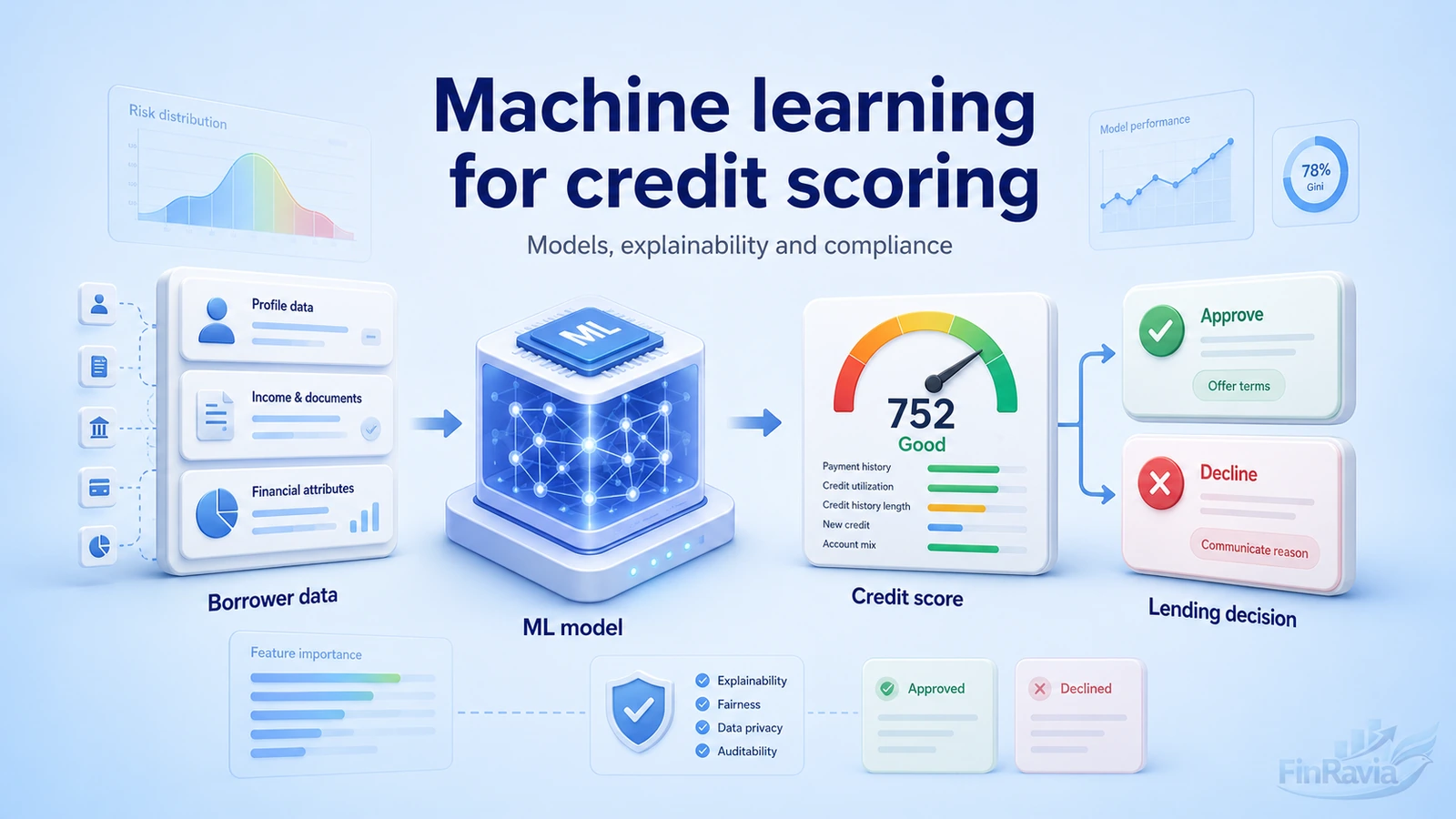
Machine Learning for Credit Scoring: Models, Benefits, Implementation, Explainability, and Compliance
Author:
Aaron Klein
Machine learning for credit scoring uses borrower, bureau, behavioral, and transaction data to predict default risk, while the 2018–2024 SLR selected 63 studies from 330 papers. Credit risk scoring still needs explainability, validation, and bias control. You will learn the models, data pipeline, metrics, SHAP logic, and compliance checks behind a deployable score.
Contents
- Why credit scoring matters in modern finance
- Business benefits of machine learning in credit scoring
- Traditional credit scoring vs ML-based credit scoring
- Financial data, target definition and feature engineering
- Machine learning model families used in credit scoring
- Practical implementation pipeline for credit scoring models
- Evaluation metrics for ML credit scoring
- Explainability, SHAP and model governance
- Compliance, regulation, privacy and responsible AI
- Evidence base, research review and model performance findings
- Case examples and real-world signals
- Common mistakes, adoption challenges and model limitations
- Future research, advanced topics and next steps
- Conclusion on machine learning for credit scoring
- Sources
Why credit scoring matters in modern finance
Financial institutions use credit scoring to process large volumes of loan applications, quantify credit risk, and support faster lending decisions.
A lender cannot price, approve, or decline credit with guesswork. Financial credit scoring turns borrower data into a structured creditworthiness assessment that measures repayment behavior, current obligations, and expected default risk.
Before standardized scoring, lending decisions depended on subjective judgment, local relationships, and manual reviews. That process created delays, inconsistent approvals, and bias that scaled badly across large portfolios.
A strong credit scoring system gives the bank a common language for borrower creditworthiness. It connects application data, repayment history, existing debt, and credit bureau records to a measurable view of risk.
An accurate credit scoring model also protects the balance sheet. It helps a bank manage credit risk exposure before approval, estimate future credit loss, and assign capital more efficiently.
| Credit scoring role | Business meaning | Risk if weak |
|---|---|---|
| Credit risk quantification | Converts borrower data into a measurable risk signal | The lender approves loans without a reliable view of default exposure |
| Borrower creditworthiness assessment | Separates stronger applicants from weaker applicants | Good borrowers can be declined while risky borrowers pass |
| Risk-based pricing | Links price, limit, and terms to expected repayment behavior | The bank underprices high-risk loans or overprices low-risk customers |
| Loan underwriting support | Gives underwriters a consistent decision framework | Manual reviews become slower, inconsistent, and harder to audit |
| Capital optimization | Helps estimate portfolio risk and expected credit loss | The institution carries risk without enough capital discipline |
| Regulation response | Creates documented logic for approval, decline, and review | The model becomes harder to defend in validation or audit |
What is credit risk and why is it difficult?
A bank asks whether a borrower will repay a loan, but credit risk modeling must handle delayed, partial, and crisis-driven repayment behavior.
Credit risk is the chance that a borrower fails to meet repayment obligations. That failure can appear as a missed payment, delinquency, restructuring, charge-off, or full loan default.
Repayment is not a clean yes-or-no event. A borrower can look safe for months and still default late. Another borrower can miss two payments, recover, and finish the loan.
Common repayment scenarios create different modeling signals:
- A customer pays 11 out of 12 months and defaults on the last month.
- A customer delays payments for 2 or 3 months and later repays the full balance.
- A customer makes no first payment after approval.
- A customer performs well until unemployment, interest rates, or an economic shock changes the default probability.
- A credit portfolio with stable past performance becomes riskier when macroeconomic stress reaches many borrowers at once.
| Repayment pattern | Modeling implication |
|---|---|
| Full repayment on schedule | Strong positive signal for future borrower performance |
| Missed payment followed by repayment | Risk signal that needs timing, severity, and recovery context |
| Late default after months of good behavior | Shows why scorecards need performance windows |
| No first payment default | Indicates fraud, severe affordability risk, or weak underwriting |
| Crisis-driven mass defaults | Requires monitoring beyond individual repayment history |
From subjective lending and FICO to machine learning
Fair Isaac Corporation introduced statistical credit scoring in 1956, replacing subjective lending with standardized borrower evaluation.
In the 1950s, credit decisions relied heavily on the judgment of a bank manager. That system worked at small scale, but it contained serious bias problems and failed when banks needed consistent approval logic across branches.
FICO changed consumer lending by turning borrower information into a standardized score. Its real value was standardization and explainability, not prediction alone.
The FICO Score assesses payment history, amounts owed, length of credit history, new credit, and credit mix. Equifax, Experian, and TransUnion later became central to standardized consumer risk evaluation.
Commercial scorecards converted borrower characteristics into points, risk bands, and approval rules. Machine learning entered this field when lenders needed richer pattern detection across larger datasets and nonlinear borrower behavior.
| Stage | Main decision logic | What changed |
|---|---|---|
| 1950s subjective lending | Bank manager judged customer character | Decisions depended on local knowledge and personal bias |
| 1956 FICO | Statistical credit scoring learned from historical credit data | Borrower evaluation became standardized |
| Commercial scorecards | Points translated borrower characteristics into risk bands | Credit teams gained repeatable approval logic |
| Logistic regression | Coefficients connected variables to default likelihood | Banks gained transparent statistical models |
| ML-based credit scoring | Algorithms detect nonlinear patterns and interactions | Lenders can assess richer data, but governance becomes stricter |
Why finance is different from generic machine learning
Financial applications differ from image classification and NLP because credit risk assessment must satisfy AUC, audit, ethics, and governance together.
In generic machine learning, a stronger model performance metric can justify a model. In finance, a high AUC is not enough. A credit model affects approval, pricing, limits, and credit denial.
A credit model can deny a borrower access to money. That decision needs an adverse action reason, documented model validation, and a governance trail that shows how data, variables, monitoring, and human review work together.
“The model said so” does not meet the standard for regulated finance.
| Generic ML success metric | Finance success metric |
|---|---|
| Higher AUC or accuracy | Predictive power plus explainability and validation |
| Model selects best pattern | Model respects regulatory constraints and business rules |
| Output only needs to be correct | Output must support review, audit, and borrower explanation |
| Black-box model can be accepted | Model governance must document data, logic, controls, and monitoring |
| Performance can dominate design | Model risk management balances accuracy, fairness, compliance, and ethics |
Business benefits of machine learning in credit scoring
Machine learning algorithms bring speed, accuracy, precision, and fairness to lending decisions by turning borrower data into measurable risk signals.
The business value of machine learning in credit scoring is not limited to a higher model score. ML affects the full lending workflow, from borrower intake and credit assessments to automated underwriting, loan processing, portfolio monitoring, and NPL management.
ML models build a more holistic borrower risk picture because they combine traditional data, behavioral signals, payment patterns, and application context.
| Benefit | Source signal | Business impact | Risk if weak |
|---|---|---|---|
| Faster lending decisions | Application data, bureau data, income verification | Shorter review cycle and cleaner routing | Manual queues delay approvals and frustrate customers |
| Better credit assessments | Repayment behavior, debt, income, alternative data | Stronger borrower profiling and sharper risk bands | Risky borrowers pass while good borrowers are declined |
| Higher operational performance | Workflow data and underwriting outcomes | Better quote speed, volume handling, and consistency | Teams scale volume without consistent quality |
| Broader financial inclusion | Thin-file data, rental records, mobile or platform income | More borrowers receive a fair review | Credit invisible applicants stay outside the system |
| Lower default rates pressure | NPL trends, loss patterns, score ranking | Better default capture and portfolio quality | Losses surface after approval instead of before |
Improve credit access and financial inclusion
Traditional credit models exclude credit invisible consumers and credit thin consumers when bureau history is too limited for standard underwriting.
More than 45 million US consumers are considered credit unserved or underserviced. The same issue appears in other markets, where large borrower groups have limited formal credit data.
Alternative data underwriting supports financial inclusion because it can read signals from rent, utilities, mobile behavior, platform income, and transaction patterns.
| Country or market | Unserved consumers |
|---|---|
| United States | Over 45 million unserved or underserviced consumers |
| India | 63% |
| South Africa | 51% |
| Colombia | 44% |
| Hong Kong | 16% |
Increase accuracy of borrower assessments
NY loan application rejection rate reached 21.8% in June 2023, making stronger borrower creditworthiness assessment more valuable.
That rejection rate was the highest since June 2018. Traditional models assess debt-to-income ratio, employment stability, repayment history, and bureau records.
ML improves assessment accuracy by adding rent payment regularity, gig-platform earning history, income volatility, and other credit risk signals. This matters because 7 in 10 UK gig workers were denied financial products despite good credit scores.
| Traditional signal | ML-added signal | What it adds |
|---|---|---|
| Debt-to-income ratio | Rent payment regularity | Shows recurring payment discipline outside credit bureau files |
| Employment stability | Gig-platform earning history | Captures income from multiple or nontraditional sources |
| Bureau repayment history | Bank transaction and cashflow patterns | Supports richer default prediction |
| Static applicant profile | Behavioral and income variability | Improves borrower profiling for irregular earners |
Accelerate decision speed and underwriting automation
Traditional financial institutions need more time for decision-making because manual review slows loan underwriting and document checks.
Closing a home loan takes 35 to 40 days on average. FinTech lenders process mortgage applications about 20% faster because they use predictive analytics, Open Banking, financial APIs, digital verification, and automated underwriting.
Kabbage reported that 95% of customers received a fully automated underwriting experience.
Operating sequence:
- Data sourcing from application, bureau, bank account, payroll, and API sources.
- Verification of income, employment, asset ownership, and identity.
- KYC background and identity checks.
- ML score for applicant risk and repayment signal.
- Underwriter summary for approval, decline, or manual review.
Drive operational performance in underwriting teams
Big data analytics and machine learning empower underwriting teams by improving quote speed, volume handling, and access to knowledge.
Many financial institutions still rely on manual credit risk assessments. Manual review affects loan underwriting because teams need to interpret documents, reconcile data, apply policy rules, and defend decisions.
| Accenture survey metric | Reported improvement |
|---|---|
| Speed to quote | 60% |
| Ability to manage large business volumes | 59% |
| Access to knowledge | 58% |
Reduce default rates and improve default capture
Every bank has quantitative NPL targets, and stronger default capture helps protect portfolio quality before losses grow.
A good non-performing loan to total asset ratio averages about 4%. Better credit loss modeling attacks the issue earlier by improving approval and ranking.
WeBank, MYBank, and XWbank issue over 10 million loans annually while maintaining an average NPL of 1%. In the BANK A case, XGBoost improved default capture against the existing score.
| NPL or default metric | Benchmark or example | Business meaning |
|---|---|---|
| Good NPL-to-total-asset ratio | About 4% | Gives banks a portfolio quality target |
| Digital bank example | WeBank, MYBank, and XWbank at 1% average NPL | Shows scalable lending with tight loss control |
| Case-by-case loss prediction | Big data plus ML | Helps price and approve borrowers by risk |
| Rank ordering | Challenger model vs incumbent score | Moves higher-risk borrowers into higher-risk bands |
Reduce manual bias and support fairer decisions
Discretionary judgments create unfair treatment when advisors rely on interviews instead of data-based decisions and controlled variables.
US minority mortgage seekers are charged 8% higher interest rates and rejected 14% more frequently. Mercado Libre uses about 2,400 behavioral variables to score applicants. Past sales history includes 250 variables and carries a 6% weight in the decision.
| Traditional evaluation | Bias risk | ML alternative | Remaining risk |
|---|---|---|---|
| In-person applicant interviews | Discretionary judgment affects approval | Structured scoring with controlled variables | Model must be tested for protected attribute proxies |
| Advisor interpretation | Similar borrowers receive different treatment | Data-based decisions with repeatable logic | Poor data can reproduce old bias |
| Limited credit history review | Thin-file borrowers are rejected early | Behavioral scoring and alternative signals | Variable weighting needs validation |
Traditional credit scoring vs ML-based credit scoring
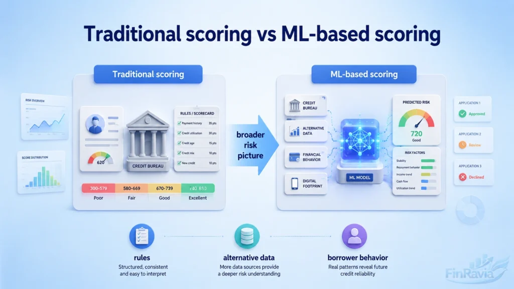
Traditional credit scoring models rely on historical credit data and fixed rules, while ML-based credit scoring uses traditional and alternative data.
Traditional systems work well when the borrower has a long repayment record, stable income, and a clean bureau file. Their strength is control. Scorecards, logistic regression, and rule-based scoring give banks a clear decision path.
The weakness appears when the borrower does not fit the old data pattern. Thin-file applicants, gig workers, new customers, and borrowers with mixed income streams can look riskier than they are.
| Area | Traditional scorecards | ML-based scoring |
|---|---|---|
| Main input | Historical credit bureau data | Bureau data plus alternative data |
| Decision logic | Pre-defined rules and points | Pattern detection and predictive risk modeling |
| Strongest use | Transparent approval rules | Broader borrower behavior analysis |
| Weak point | Limited view of thin-file borrowers | Needs validation, governance, and explainability |
| Business output | Stable score bands | More granular credit risk ranking |
Data sources: credit bureaus, FICO, VantageScore and alternative data
Equifax, Experian, and TransUnion provide credit bureau data that supports FICO, VantageScore, and many lender scoring systems.
FICO Score and VantageScore use historical agency data to assess repayment patterns. Traditional systems use about 10 to 20 assessment criteria.
Alternative credit data includes rent and utility payments, cashflow trends, checking account information, mobile payments, telecom data, and Internet behavior.
| Traditional data source | Alternative data source | Scoring value |
|---|---|---|
| Bureau repayment record | Rent and utility payments | Shows payment discipline outside credit cards and loans |
| Employment records | Gig-platform income | Captures nontraditional earning patterns |
| Lending history | Checking account cashflow | Supports affordability and liquidity analysis |
| Credit account data | Mobile and telecom data | Adds behavioral signals for thin-file borrowers |
| Static application fields | Mobile usage and transaction behavior | Improves borrower context before underwriting |
Scorecards and logistic regression as traditional baseline
Banks still use logistic regression because it estimates default probability with transparent coefficients and regulator-friendly model logic.
Logistic regression classifies a binary outcome. Risk teams can explain why a variable increased or reduced risk because every coefficient has a direction and size.
A scorecard translates logistic regression into a business tool. Weight of Evidence supports binning and variable transformation, while PDO defines how many points double the odds.
| Scorecard component | Function |
|---|---|
| Binning | Groups borrower features into interpretable ranges |
| Weight of Evidence | Converts category risk into a usable model signal |
| Points allocation | Turns model effects into scorecard points |
| Total score | Sums all points into a single score |
| PDO | Defines points needed to double the odds |
| Score | Default probability |
|---|---|
| 400 | 9.09% |
| 500 | 4.76% |
| 600 | 2.44% |
| 700 | 1.23% |
| 800 | 0.62% |
A 100-point increase approximately halves default probability, which gives underwriters and policy teams a direct way to connect score bands with risk.
Limitations of logistic regression and traditional scorecards
Traditional models struggle with nonlinear borrower behavior because logistic regression does not learn complex patterns on its own.
Age can create a U-shaped risk relationship, and interactions make the problem heavier. With 20 features, the model can create 190 possible pairwise interactions.
| Limitation | Example | Workaround | Remaining risk |
|---|---|---|---|
| Non-linear relationships | Age-risk pattern becomes U-shaped | Add bins or age² term | Manual design can miss real patterns |
| Missing interactions | Income and short credit history interact | Add interaction terms | 20 features create 190 pairs |
| High-dimensional data | Alternative data creates hundreds of variables | Feature selection and grouping | Overfitting remains possible |
| Multicollinearity | Related transaction variables move together | Remove or combine correlated features | Model stability can still weaken |
Financial data, target definition and feature engineering
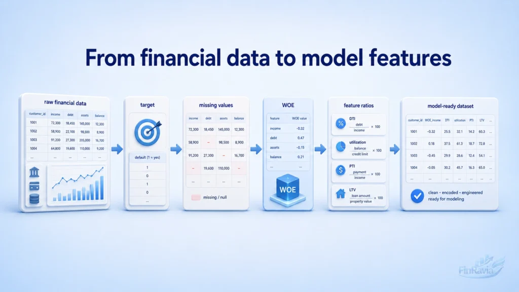
Financial data differs from generic ML datasets because borrower records contain imbalance, time effects, missing values, and regulatory limits.
A credit model learns from applications, bureau records, payments, income, debts, behavioral signals, and portfolio outcomes. That makes feature engineering central to the model.
| Data issue | Example | Modeling risk | Mitigation |
|---|---|---|---|
| Class imbalance | Defaults are rare compared with good accounts | Model learns to predict everyone as good | Use PR, recall, class weights, resampling, and rank-order checks |
| Censored data | Rejected applicants have no repayment outcome | Model sees only accepted borrowers | Use reject inference controls and document accepted-borrower bias |
| Missing values | No bureau field, no income record, no account age | Missingness can carry risk information | Add missingness flags or use models that route missing values |
| Temporal dependency | Old repayment data shifts under new economic stress | Model drift weakens decisions | Use out-of-time validation and monitoring |
| Regulatory limits | Protected traits and proxies enter variables | Legal and fairness risk | Remove prohibited variables and test proxy behavior |
Target variable and performance window
The target variable is defined as ever 60 day past due or worse within the first 18 months after origination.
This binary target includes charge-offs and repossessions. Development records that meet the delinquency target receive target value 0 and are labeled Bad. All other records receive target value 1 and are labeled Good.
| Condition | Target value | Label |
|---|---|---|
| Ever 60 days past due or worse within first 18 months | 0 | Bad |
| Charge-off within first 18 months | 0 | Bad |
| Repossession within first 18 months | 0 | Bad |
| No qualifying bad event in the performance window | 1 | Good |
Unique challenges of financial data
A well-functioning credit portfolio has a 1–5% default rate, so class imbalance can make a useless model look accurate.
A naive model that predicts every borrower will pay can exceed 95% accuracy and still miss every default. Credit risk also has temporal dependency because unemployment, interest rates, and economic cycles change borrower behavior.
A model cannot use race, gender, or religion. A variable such as zip code can still correlate with race, which creates proxy discrimination and legal exposure.
| Challenge | Example | Modeling risk | Mitigation |
|---|---|---|---|
| Rare defaults | 1–5% default rate | Accuracy hides missed defaults | Use PR, recall, KS, decile analysis |
| Model drift | Crisis, unemployment, rate changes | Old patterns lose predictive power | Add out-of-time validation and monitoring |
| Reject inference | Only accepted borrowers have outcomes | Training data misses declined applicants | Track approval policy and accepted-borrower bias |
| Protected traits | Race, gender, religion | Direct discrimination | Exclude prohibited variables |
| Proxy variables | Zip code correlates with race | Indirect discrimination | Test proxy behavior and document removals |
Data preprocessing, missing values and outliers
Missing values are often informative in finance because “no information” can signal risk, thin files, or incomplete borrower history.
⚠️ No imputation performed best in the BANK A XGBoost case because XGBoost handles missing values inside tree splits. Some models still need median filling, missingness flags, or separate categories.
Outliers need care. Winsorization keeps the record and caps numeric columns at quantile limits, which is safer than removing real extreme borrowers.
| Flow step | Treatment | Purpose |
|---|---|---|
| Raw data | Keep original borrower fields | Preserve the first risk signal |
| Missing handling | Use missingness flag, median filling, or XGBoost default routing | Decide whether absence itself predicts risk |
| Feature creation | Build DTI, utilization, account-age and payment features | Convert raw fields into credit logic |
| Outlier handling | Cap numeric columns at quantile limits | Limit extreme influence without deleting records |
| Processed dataset | Validate distributions and model performance | Confirm preprocessing improves model behavior |
Categorical encoding and Weight of Evidence
The model uses WOE encoding for categorical features by comparing good ratios and bad ratios inside each category.
🧮 Formula: WOE = ln(distribution of Goods / distribution of Bads)
| WOE value | Interpretation |
|---|---|
| Below 0 | Category leans toward higher bad-rate behavior |
| Near 0 | Category is close to neutral |
| Above 0 | Category leans toward higher good-rate behavior |
Domain-driven features and variable selection
Reviewed studies used demographic, financial, behavioral, and transaction-level variables for credit scoring.
| Variable category | Examples | Credit scoring meaning |
|---|---|---|
| Demographic variables | Age, marital status, employment type, dependents, residence type | Describes borrower background, subject to fairness controls |
| Financial variables | Annual income, loan amount, monthly payment, debt, account balance | Measures capacity and current obligations |
| Behavioral variables | Payment history, late payments, credit utilization, repayment patterns | Captures past borrower performance |
| Transaction-level variables | Cashflow, deposits, withdrawals, account activity | Shows current financial behavior |
| Feature ratio | Formula | Risk meaning |
|---|---|---|
| DTI | Debt / Income | Measures debt burden against income |
| Utilization | Credit used / Credit limit | Shows pressure on available revolving credit |
| PTI | Payment / Income | Measures payment affordability |
| LTV | Loan amount / Collateral value | Measures secured-loan exposure against collateral |
Variable selection improves model performance by identifying relevant variables and reducing noise. In the BANK A case, XGBoost feature importance and Shapley score supported final feature reduction.
Machine learning model families used in credit scoring
Machine learning algorithms include supervised, unsupervised, and semi-supervised learning for credit scoring models.
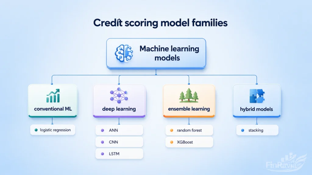
| ML layer | Model family | Typical role in credit scoring |
|---|---|---|
| Machine learning models | Conventional ML | Transparent baseline models for borrower default prediction |
| Machine learning models | Deep learning | Complex predictive models for high-dimensional or sequential data |
| Machine learning models | Ensemble learning | Stronger classification through combined learners |
| Machine learning models | Hybrid models | Integrated systems for imbalanced data, segmentation, and optimization |
| Learning setup | Supervised learning | Learns from labeled default and non-default outcomes |
| Learning setup | Unsupervised learning | Finds applicant groups without predefined labels |
| Learning setup | Semi-supervised learning | Uses limited labels with broader unlabeled borrower data |
Logistic regression
Logistic regression makes binary predictions by estimating borrower default probability on a 0 to 1 probability scale.
It remains a strong baseline because the output is interpretable, the coefficients show direction, and the method resists noise in smaller datasets. Cao et al. set the optimal probability threshold at 0.18 through Youden’s index and reached 86.58% accuracy.
| Study or example | Dataset or context | Metric | Limitation |
|---|---|---|---|
| Cao et al. | Credit score and default probability model | 0.18 threshold and 86.58% accuracy | Threshold depends on validation goal |
| Portuguese model | Financial institution credit data | 89.79% correct default prediction | Works best when relationships stay stable |
| PLTR | Logistic regression plus decision-tree rules | Keeps interpretability and captures nonlinear effects | More complex than standard LR |
| Standard LR | Smaller labeled credit datasets | Clear interpretable credit scoring | Linear log-odds assumption |
Decision trees and CART
Decision trees forecast future observations by splitting borrower data into high-risk and low-risk loan groups.
A tree starts with a root, applies a decision rule, follows a branch, and ends at a leaf that represents the final prediction.
Simple tree diagram:
Applicant → repayment history clean → utilization below risk threshold → lower-risk score band
| Tree strength | Limitation | Mitigation |
|---|---|---|
| Clear classification rules | Deep trees overfit training data | Limit depth and validate out of time |
| Natural risk segmentation | Small data changes alter splits | Use pruning or ensemble models |
| Captures nonlinear patterns | Single tree can be weak | Use random forest or gradient boosting |
| Easy review by underwriters | Split logic can become fragmented | Keep policy documentation |
Khedr’s model reached almost 94.85% accuracy, while C4.5 achieved 85.23% F1-score and 78.33% accuracy.
Random forest
Random forest aggregates multiple decision trees and predicts through majority vote across an uncorrelated forest.
Random forests handle high-dimensional data, reduce overfitting compared with individual trees, and assign variable importance. They also handle missing data.
Mini-scheme: many resampled datasets → many trees → majority vote → final score
| Advantage | Limitation |
|---|---|
| Stronger prediction than one tree | Harder to explain individual decisions |
| Lower overfitting risk than a deep tree | More computation than a small model |
| Handles missing data and many variables | Requires careful validation of feature importance |
| Supports robust prediction | Can hide weak data quality behind aggregate performance |
RF plus chi-square reached 93.12% accuracy and 93.10% F1-score. NCSM optimized RF through feature selection and grid search.
Support vector machine and K nearest neighbors
SVM maps borrower data into high-dimensional space and separates default and non-default classes with a hyperplane.
SVM reached 98.34% classification accuracy in one comparison, and IFOA-SVM reached 93% precision. KNN uses a distance function and selected k value to classify a borrower by nearby cases.
| Algorithm | How it works | Best use | Risk |
|---|---|---|---|
| SVM | Finds a separating hyperplane in high-dimensional space | Clear default versus non-default classification | Kernel tuning increases cost |
| IFOA-SVM | Optimizes SVM parameters | Higher precision settings | More complex validation |
| K nearest neighbors | Classifies by nearest borrower records | Borrower similarity tasks | Slow with large datasets |
| k-NN with k=1 | Uses the nearest case | Low-error benchmark cases | Sensitive to noise |
Gradient boosting, GBDT and XGBoost
Boosting learns a sequence of weak predictors and improves credit classification by minimizing previous errors.
XGBoost extends gradient boosting with speed, parallelization, and a stronger objective function. Its objective combines loss and a regularization term.
- Initialize a baseline prediction.
- Fit a weak tree to current errors.
- Compute pseudo residuals through negative gradient.
- Add the next tree to reduce loss.
- Apply regularization to control complexity.
- Validate AUC, PR, KS, calibration, and out-of-time behavior.
| Gradient boosting | XGBoost |
|---|---|
| Builds trees sequentially | Uses optimized and parallelized tree boosting |
| Minimizes loss with additive trees | Combines loss and regularization term |
| Captures nonlinear patterns and interactions | Adds overfitting control and faster training |
| Strong predictive baseline | Stronger production candidate when governance is handled |
| Model | AUC or AUROC | Interpretation |
|---|---|---|
| Logistic regression in synthetic tutorial | 0.6842 | Missed nonlinear and interaction effects |
| Gradient boosting in synthetic tutorial | 0.7651 | Captured nonlinear and interactive risk structure |
| BANK A incumbent model | 0.77 OOT AUROC | Existing benchmark score |
| XGBoost challenger model | 0.80 OOT AUROC | Better out-of-time separation |
Deep learning with ANN, DNN, CNN and LSTM
Deep learning is a subset of ML where neural networks with multiple layers extract patterns from complex credit data.
ANN models extract features automatically, which helps with larger datasets, but they create interpretation challenges in regulated lending. LSTM models handle variable-length sequential data and fit payment sequences.
| Model | Data type | Use case | Metric or limitation |
|---|---|---|---|
| ANN | Structured borrower data | Automatic feature extraction | 91.91% accuracy and 92.60% AUC in Kazemi model |
| DNN | Text, image, audio, video | Statement verification, OCR, NLP | Strong pattern extraction, weak interpretability |
| CNN | Image-like credit features | Classification from transformed tabular data | 95.00% accuracy in one 2D CNN study |
| LSTM | Payment sequence and behavior history | Missed payments and behavioral scoring | 90.69% accuracy and 91.00% AUC in transactional data |
Hybrid, composite and ensemble models
Hybrid models integrate multiple algorithms to improve predictive performance, feature selection, and segmentation in credit scoring.
| Model family or components | Dataset or context | Best metric | Limitation |
|---|---|---|---|
| RF-SVM | Ensemble with RF feature selection and SVM classifier | 87.94% accuracy and 92.10% AUC | More complex than either model alone |
| MHS-RF | Harmony Search plus random forest | 87.38% accuracy | Requires optimization control |
| SOM + CART | Clustered inputs fed into CART | CART improved from 96.30% to 96.70% | Segmentation logic needs monitoring |
| DGHNL | Evolutionary computation, ensemble learning, deep learning | 97.39% accuracy on Australian dataset | High model complexity |
| Shen model | LSTM, AdaBoost, enhanced SMOTE | 80.32% AUC | Imbalance treatment affects calibration |
| He model | BalanceCascade, RF, XGBoost, stacking, PSO | 92.79% AUC | Layered validation burden |
| GSCI | Shapley Choquet Integral ensemble | 94.53% recall, 90.91% F1-score, 91.43% AUC | Explanation and governance are heavier |
| Stacked ensemble | RF, XGBoost, TabNet | Integrated ensemble score | Requires strong monitoring and documentation |
Practical implementation pipeline for credit scoring models
An ML project for credit scoring has three major steps, from preprocessing to model training and validation.
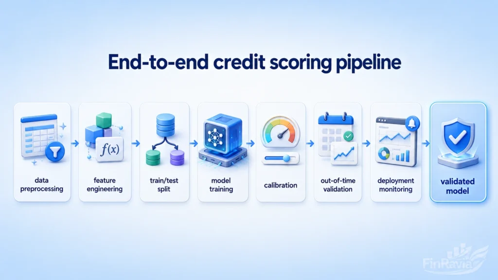
A deployable implementation pipeline begins with raw borrower data, a clean target, controlled features, and a validation design that shows how the model behaves outside the training sample.
Full process flow:
Raw applications → data preprocessing and feature engineering → target definition and sample split → model specifications → model building and training → model comparison → model calibration and fine tuning → out-of-time validation → monitoring and deployment
Model development tools and dependencies
The BANK A model was developed in Python 3.7 with datasets provided as CSV files.
| Package | Purpose |
|---|---|
| numpy | Numerical computation |
| pandas | Data manipulation and tabular preparation |
| scikit-learn | Splits, metrics, preprocessing, and baseline models |
| xgboost | XGBoost model training |
| category-encoders | Categorical feature encoding |
| joblib | Model serialization |
| tqdm | Progress tracking |
| matplotlib and seaborn | Visualization |
| scikitplot | Model plots |
| shap | Explainability library |
Model training, cross-validation and calibration
Cross-validation assesses ML method quality by testing candidate settings across repeated training and validation splits.
In k-fold cross-validation, one subsample becomes validation data and the remaining k−1 subsamples become training data. The tutorial example uses a train/test split with a 25% test size.
| Metric | Model phase | Purpose | Risk if misused |
|---|---|---|---|
| ROCAUC | Training and cross-validation | Measures class separation | Can look strong when defaults are rare |
| Log-Loss | Training and calibration | Penalizes poor probability separation | Can push probability behavior without business threshold checks |
| Fβ-score | Hyperparameter tuning | Weights precision and recall | Wrong β shifts focus away from default capture |
| Reliability curve | Calibration | Tests probability confidence interpretation | Poor calibration makes PD-style use unsafe |
| Gini | Model comparison | Converts AUC into finance metric | Does not replace out-of-time validation |
Class imbalance, loss reweighting and resampling
Class imbalance is common in credit portfolios because good borrowers outnumber defaulting borrowers.
⚠️ Reweighted model score does not equal real default probability. Loss reweighting changes the probability measure, so the model can support rank ordering but not direct real-world probability interpretation without calibration.
| Imbalance method | Benefit | Drawback |
|---|---|---|
| Class weights | Raises penalty for missed defaults | Changes optimization pressure |
| Loss reweighting | Emphasizes the minority class | Changes the probability measure |
| Oversampling | Adds more minority-class cases | Prone to overfitting |
| Under-sampling | Reduces majority-class dominance | Removes useful good-borrower data |
| SMOTE | Creates new minority instances | Synthetic records can weaken calibration |
| PR curve | Complements AUC under imbalance | Needs business interpretation |
Final model form, hyperparameters and conservative controls
The final model appends important features to the original thirteen Credit Bureau B features.
| Parameter | Role | Higher value effect | Credit scoring implication |
|---|---|---|---|
| alpha | L1 regularization | More conservative weights | Reduces noisy feature influence |
| lambda | L2 regularization | Smoother model | Limits unstable weight growth |
| gamma | Minimum split gain | Fewer splits | Helps control overfitting |
| max_depth | Maximum tree depth | More complex trees | Captures interactions but raises validation burden |
| learning_rate | Shrinks feature weights | Slower learning | More controlled boosting |
| scale_pos_weight | Balances class weights | Stronger minority-class pressure | Helps imbalanced default data |
| max_delta_step | Leaf output constraint | More conservative updates | Limits extreme class-imbalance behavior |
| subsample | Row sampling | More randomness | Helps prevent overfitting |
Out-of-time validation, decile analysis and swap set analysis
Decile analysis divides customers into 10 groups ordered by predicted risk to test default capture.
| OOT metric | Our model | BANK A model |
|---|---|---|
| KS statistic | 44.91 | 41.31 |
| AUROC | 0.80 | 0.77 |
| PR curves value | 0.093 | 0.06 |
| Risk segment | Our model bads | BANK A bads | Business reading |
|---|---|---|---|
| Worst 20% | 5157 | 4748 | Challenger captures more high-risk accounts |
| Worst 10% | 3561 | 3065 | Challenger concentrates more defaults in the riskiest band |
| Decile | Predicted risk band | Count | Defaults | Default rate | Capture rate | Cumulative capture |
|---|---|---|---|---|---|---|
| 1 | Highest risk | Add portfolio count | Add bad count | Add rate | Add share | Add cumulative share |
| 10 | Lowest risk | Add portfolio count | Add bad count | Add rate | Add share | Add cumulative share |
Evaluation metrics for ML credit scoring
Metric selection is critical in credit scoring because a model with high accuracy can still miss every default.
| Confusion matrix cell | Meaning in credit scoring |
|---|---|
| True positive | Model correctly flags a borrower as default risk |
| True negative | Model correctly identifies a borrower as non-default |
| False positive | Model flags a good borrower as risky |
| False negative | Model treats a risky borrower as good |
| Metric | What it measures | When useful | Weakness |
|---|---|---|---|
| Accuracy | Overall correct predictions | Balanced datasets | Misleads on imbalanced datasets |
| Precision | Correctness among predicted defaults | Manual review queues and risk alerts | Can look good while missing many defaults |
| Recall | Share of real defaults caught | Default detection and loss control | Can rise by flagging too many good borrowers |
| F1-score | Balance of precision and recall | Single summary for imbalanced classification | Hides business cost differences |
| AUC | Class separation across thresholds | Model ranking and comparison | Does not show calibration |
| Gini | Finance version of AUC separation | Credit risk reporting | Same blind spots as AUC |
| KS statistic | Maximum separation between good and bad distributions | Scorecard and credit model validation | Needs distribution review |
| PR curve | Precision-recall trade-off | Rare default events | Harder to compare across portfolios |
| Log-Loss | Probability error | Calibration and probability quality | Can conflict with simple rank-order goals |
AUC and PR should be used together in imbalanced contexts because a clean headline metric can hide weak default capture.
Explainability, SHAP and model governance
Complex models often lack interpretability, so explainability now determines whether a credit model can pass governance review.
| Explanation method | What it answers | Compliance value |
|---|---|---|
| Coefficients | Which direction a variable moves risk | Useful for transparent statistical models |
| LIME | Which local variables influenced one prediction | Gives a local explanation for a borrower case |
| SHAP | How each feature contributed to model output | Supports local and global explanation with additive attribution |
| Feature importance | Which variables matter most overall | Helps model review, but not adverse action reasons alone |
| Partial dependence | How a variable affects predictions across values | Supports model behavior review |
| Documentation and monitoring | Whether explanations stay stable over time | Supports model governance and audit trail |
Logistic regression explainability vs gradient boosting explainability
Logistic regression coefficients are directly interpretable because each coefficient shows the direction and size of a risk effect.
| Explanation layer | What it gives | What it misses |
|---|---|---|
| Logistic regression coefficient | Direction and size of feature effect | Limited nonlinear behavior |
| GB feature importance | Global ranking of influential variables | No direction, threshold, or local reason |
| Partial dependence | Average variable behavior | Weak for individual denial explanation |
| SHAP | Local explanation and global explanation | Needs governance controls and reviewer training |
Shapley values and additive feature attribution
An explanation model is an interpretable approximation of the initial model for one prediction or a simplified input space.
📌 Definition box:
- Local methods explain a single borrower prediction.
- Additive feature attribution assigns one contribution value to each feature.
- The sum of attributions approximates the original model output.
- Shapley Values come from cooperative game theory.
| Property | Meaning | Compliance value |
|---|---|---|
| Local accuracy | Explanation output matches the original prediction for the borrower | Supports borrower-level review |
| Missingness | Missing features receive no contribution | Prevents fake reasons from entering the explanation |
| Consistency | Attribution does not fall when feature contribution rises | Protects explanation logic from contradictory behavior |
| Uniqueness theorem | One solution satisfies the attribution rules | Makes the method more defensible in validation |
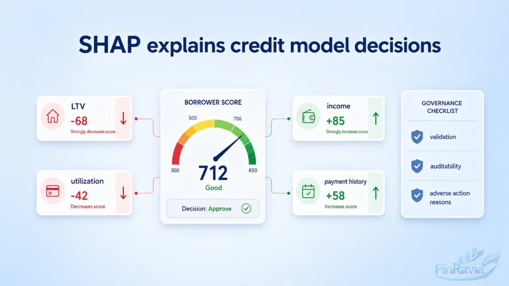
SHAP plots and practical credit score explanations
SHAP explains ML and DL model output by connecting game theory with local additive explainers.
In the BANK A case, low APR and low LTV pushed a high score upward. Bankcard Revolving, Transactor, and Inactive patterns drove a low score.
| SHAP plot type | Use case | Answer it gives |
|---|---|---|
| Summary plot | Portfolio-level model review | Which features matter most across borrowers |
| Dependence plot | Variable behavior analysis | How feature values change SHAP contribution |
| Force plot | Single applicant review | Which factors moved one score up or down |
| SHAP values table | Audit and documentation | Exact feature contribution behind the score |
| Interaction review | Nonlinear model inspection | Which variables work together inside the model |
Compliance, regulation, privacy and responsible AI
Regulated banking context limits practical ML model usage because compliant credit scoring must document design, validation, fairness, and data controls.
The compliant approach introduces BASEL 2 and BASEL 3 techniques, answers Federal Reserve and ECB requirements, and connects XGBoost performance with Shapley-based explanations.
✅ Compliance checklist:
- Document model purpose, portfolio, data, target, variables, and decision use.
- Validate discrimination, calibration, stability, out-of-time behavior, and reject logic.
- Explain model outputs with SHAP, adverse action logic, or another auditable method.
- Remove prohibited variables and test proxy behavior.
- Protect sensitive records through data security, access control, privacy safeguards, and cybersecurity.
| Regulation or framework | Requirement | Article section that covers it |
|---|---|---|
| BASEL 2 and BASEL 3 | Model documentation, validation, and capital discipline | Implementation pipeline, validation, model governance |
| SR 11-7 | Model risk management and independent validation | Model governance and validation framework |
| OCC Bulletin | Auditable model design and control evidence | SHAP, explainability, conservative controls |
| Federal Reserve requirements | Model governance and supervisory defensibility | Compliance and model auditability |
| ECB requirements | Validation discipline in regulated banking | Out-of-time validation and governance controls |
| IFRS 9 | Expected Credit Loss estimation through PD, EAD, and LGD | Evaluation metrics and portfolio risk use |
| Fair Credit Reporting Act | Limits features that create impermissible credit decision logic | Variable selection and fairness review |
Regulatory uncertainty and model risk management
Financial regulations were created before the proliferation of ML, so automated credit models face regulatory uncertainty.
⚠️ Regulatory risk checklist:
- Does the model support the exact credit decision it influences?
- Does the validation file explain inputs, target, features, thresholds, and limitations?
- Does automated decisioning produce usable adverse action reasons?
- Does monitoring detect drift, bias, and performance decay?
- Does a policy owner control when the model can be changed or retired?
Bias, fairness and proxy discrimination
Machine learning models require representative datasets because flawed data can aggravate credit accessibility issues.
Process diagram: original decision → remove protected attributes → rerun borrower evaluation → compare outcome → flag biased case if approval changes
| Fairness risk | Where it appears | Control |
|---|---|---|
| Flawed data | Thin-file and underserved applicants missing from training data | Representative sampling and bias review |
| Sample bias | Accepted borrowers dominate observed outcomes | Reject inference controls |
| Protected trait use | Race, gender, or religion enters the model | Remove prohibited fields |
| Proxy variables | Zip code or behavior pattern mirrors protected groups | Proxy testing and fairness monitoring |
| Biased approval logic | Approval changes after protected attributes are removed | DualFair-style rerun and case flagging |
Data security and privacy risks
ML models need access to sensitive customer data for underwriting, which makes data security a credit-risk control.
| Data risk | Consequence | Mitigation |
|---|---|---|
| Excessive data collection | Privacy risk and weaker borrower trust | Data minimization and purpose limits |
| Re-identification | Anonymized data becomes linkable to a person | Strong anonymization and access controls |
| Inferred protected traits | Model learns age, race, or gender indirectly | Proxy testing and protected-trait review |
| Cyberattack risk | Customer files and decision logs are exposed | Secure lending infrastructure and monitoring |
| Limited data availability | Model loses signal or becomes biased | Document gaps and validate performance by segment |
Evidence base, research review and model performance findings
The systematic literature review covers ML-based financial credit scoring methods from 2018 to 2024 and synthesizes 63 primary studies.
Researchers extracted 330 research papers, while database searches and snowballing identified 345 studies before screening. Included studies comprised 48 journal articles and 13 conference papers.
| Review element | Value |
|---|---|
| Period covered | 2018–2024 |
| Initial extracted papers | 330 research papers |
| Database searches plus snowballing | 345 studies |
| Final synthesis | 63 primary studies |
| Publication types | 48 journal articles and 13 conference papers |
| Frequent public datasets | German, Australian, and Japanese datasets |
| Proprietary data use | About one-third of studies |
🔎 PRISMA flow diagram: identification → 345 studies found → screening → eligibility review → quality assessment → 63 primary studies included.
| Ranked evidence item | What it compares | Why it matters |
|---|---|---|
| Tables 4–6 | Models, datasets, and metrics | Shows the research base behind each method |
| Tables 7–10 | Ranked accuracy and AUC results | Gives a compact view of top-performing methods |
| Citation analysis | Influential studies and intellectual links | Shows which papers shape the field |
| Scientific mapping | Conceptual clusters and keyword links | Shows how the research area is organized |
Methodology of the systematic review
The SLR adheres to PRISMA 2020 guidelines and uses predefined research questions to structure the review.
| Research question | What it asks |
|---|---|
| RQ1 | Most widely used ML models |
| RQ2 | Strengths and limitations of ML models |
| RQ3 | Evaluation metrics used in credit scoring |
| RQ4 | Emerging trends and advances |
| RQ5 | Adoption challenges |
| PRISMA item | Applied in review |
|---|---|
| Reporting guidance | PRISMA 2020 used |
| Protocol registration | Formal PROSPERO registration not undertaken |
| Identification | Four digital libraries used |
| Screening | Duplicates and irrelevant papers removed |
| Eligibility | Criteria applied to publication type, language, period, and empirical results |
| Inclusion | 63 studies entered synthesis |
| Inclusion criteria | Exclusion criteria |
|---|---|
| Publication between 2018 and 2024 | Studies before 2018 |
| English language | Duplicates |
| Empirical results | Papers under 4 pages |
| ML credit scoring focus | Incomplete or non-transparent studies |
| Peer-reviewed journal or conference paper | Articles without metrics |
| Addressed at least one RQ | Studies outside the RQ scope |
The data extraction form was implemented as an Excel spreadsheet. Selected studies achieved at least a 77% quality threshold.
Prior reviews and literature gaps
Related work shows that earlier literature reviews found strong ensemble performance but left gaps in interpretability, imbalance, and datasets.
| Prior review | Scope | Strongest models | Limitations |
|---|---|---|---|
| Dastile et al. | 74 studies from 2010–2018 | RF, XGBoost, CNN | Lack of macroeconomic variables |
| Kumar et al. | Rural finance and fintech | ANN, SVM, RF, hybrid approaches | Performance analysis stayed more conceptual |
| Hayashi | DL in credit scoring from 2019–2022 | DBN and CNN | Interpretability remained difficult |
| Lenka et al. | Ensemble learning for imbalanced data | GA feature selection and CatBoost | Focused strongly on imbalance methods |
| Markov et al. | Historical model shift | SVMs, ensembles, neural networks | Less focus on recent explainability tools |
| Kamimura et al. | Optimization methods | Hybrid models at 72% in reviewed methods | Calls for more legal, ethical, and practical work |
Comparative performance results across studies
Performance analysis shows that hybrid and ensemble approaches deliver stronger results than traditional LR and SVM in many reviewed comparisons.
| Model or approach | Dataset or context | Reported metric | Reading |
|---|---|---|---|
| GA + NN | German dataset | 91.91% accuracy and 92.60% AUC | Strong hybrid ML result |
| Zhang multi-stage ensemble | Australian and Japanese datasets | Outperformed other methods | Strong benchmark performance |
| GSCI model | Lending Club | Led performance | Strong ensemble result |
| Random Forest and hybrid ML | ML comparison | Highest ML accuracies | Strong conventional and hybrid signal |
| CNN and hybrid DL | DL comparison | Robust performance | Good fit where feature representation is controlled |
| Scientific mapping item | Result | Meaning |
|---|---|---|
| Bibliographic coupling | Three conceptual clusters | Shows linked research streams |
| Keyword co-occurrence | Six thematic clusters | Shows recurring themes across ML credit scoring |
| VOSviewer mapping | Network structure | Connects studies, methods, and research topics |
Case examples and real-world signals
BANK A used an auto loan scoring model, and XGBoost challenged it with stronger default capture.
| Company or case | Data or model | Metric or result | Article use |
|---|---|---|---|
| BANK A | Auto loan applicant scoring model | XGBoost challenger beat the incumbent score on OOT separation | Shows governed challenger-model testing |
| BANK A challenger | XGBoost plus Shapley explanations | Better default capture than the original model | Supports the explainability and governance sections |
| SoFi | Education, utility, insurance, and mobile signals | 584K new customers added in Q2 2023 | Shows alternative data in consumer lending |
| Kabbage | Automated underwriting workflow | 95% fully automated underwriting experience | Shows speed and workflow automation |
| WeBank, MYBank, XWbank | Big data and digital bank scoring | Over 10 million loans annually with 1% average NPL | Shows portfolio-scale loss control |
| Mercado Libre | 2,400 behavioral variables | Past sales history has 250 variables and 6% decision weight | Shows behavioral scoring in platform lending |
| Bank of America | NLP for corporate credit analysis | Corporate text becomes risk signal | Shows NLP use beyond consumer scoring |
Common mistakes, adoption challenges and model limitations
ML models introduce operational risks when data leakage, weak metrics, and feature mistakes pass validation.
⚠️ Do not deploy before checking:
- The training data contains no future information.
- The validation split follows time, not random convenience.
- The metric set covers AUC, Gini, KS, PR, recall, and decile behavior.
- The features encode credit logic, not raw noise.
- The model has bias, privacy, drift, and monitoring controls.
- The score is used only inside the approved implementation scope.
Data leakage and temporal validation
Data leakage trains a credit model with future information, making the validation result stronger than real performance.
| Split type | Example | Reading |
|---|---|---|
| Wrong split | Shuffle all rows and split randomly | Creates look-ahead bias |
| Correct split | Train on 2020–2022 and test on 2023 | Tests real future performance |
| Deployment split | Use out-of-time validation by application date | Prevents temporal leakage |
Optimizing the wrong metric
Accuracy is misleading with imbalanced data because a naive classifier can predict everyone will pay.
| Metric | What it captures | When to use |
|---|---|---|
| AUC-ROC | Discriminatory power across thresholds | Model ranking |
| Gini coefficient | Finance-readable AUC transformation | Credit score comparison |
| KS Statistic | Maximum good-bad separation | Scorecard validation |
| PR curve | Default detection under imbalance | Rare default portfolios |
| Decile analysis | Business concentration of defaults | Underwriting and portfolio review |
Lack of domain knowledge in feature engineering
Raw features are weaker than meaningful ratios because borrower affordability depends on relationships between values.
| Ratio | Formula | Credit meaning |
|---|---|---|
| DTI | Debt / Income | Measures debt burden |
| Utilization | Credit used / Credit limit | Measures revolving credit pressure |
| PTI | Payment / Income | Measures payment affordability |
| LTV | Loan amount / Collateral value | Measures secured-loan exposure |
Curse of dimensionality and feature explosion
High-dimensional data increases computational demands and weakens model generalization when sparse variables dominate.
| Feature selection method | How it works | Best fit |
|---|---|---|
| Filter methods | Rank variables before model training | Fast screening of high-dimensional data |
| Wrapper methods | Test variable subsets with model feedback | Smaller feature sets with performance checks |
| Embedded methods | Select variables during model training | Tree models, regularized models, and XGBoost |
| Manual credit review | Removes features with weak business logic | Fairness, policy, and explainability control |
Behavioral and attitudinal data integration
Loan repayment is influenced by ability and willingness to repay, not only by income and bureau history.
| Ability indicators | Willingness indicators |
|---|---|
| Income and cashflow | Repayment priority |
| DTI and PTI | Financial knowledge |
| Utilization | Debt attitude |
| Employment stability | Integrity indicators |
| Collateral and LTV | Lifestyle and gratification signals |
Model scope, use restrictions and limitations
The BANK A model was designed using auto loan origination data and customer records with Fico 8 Auto above 660.
| Assumption or limitation | Implementation consequence | Risk if violated |
|---|---|---|
| Auto loan origination data | Use the score for loan origination only | Model logic fails in account management |
| Fico 8 Auto above 660 | Keep the score inside the approved score band | Applicants outside scope receive unstable scores |
| Class reweighting | Treat output as rank order, not real PD | Pricing or capital use becomes misleading |
| No default probability output | Add calibration before PD-style use | Probability language becomes inaccurate |
| Missing imputation changes output | Preserve tested missing-value treatment | Model behavior shifts after deployment |
Future research, advanced topics and next steps
Future research should establish standardized benchmarking protocols and build privacy-safe alternative data use into credit scoring.
| Future research agenda | What it studies | Credit scoring value |
|---|---|---|
| Standardized benchmarking | Shared datasets, metrics, and validation protocols | Makes model results comparable |
| Privacy-safe alternative data | Telecom, e-commerce, and social media signals | Expands borrower view without uncontrolled privacy risk |
| Survival analysis | When default will occur | Adds time-to-default insight |
| Reject inference | Learning from rejected applications | Reduces accepted-borrower bias |
| Stress testing | Model behavior under economic shocks | Tests resilience under crisis conditions |
| Time series plus ML | Macroeconomic factors and borrower performance | Connects risk scores with economic cycles |
| Graph neural networks | Customer relationship networks | Learns connected borrower and transaction structure |
| Transformers | Time series and text data | Processes sequences, documents, and credit narratives |
| Further reading | Basel, SR 11-7, SHAP, model validation, fairness testing | Deepens governance and deployment quality |
Regulatory and risk-management depth
Basel regulations define requirements for banks using own models, and the IRB approach links those models to capital calculations.
| Concept | Meaning | Why it matters |
|---|---|---|
| Basel regulations | Banking rules for capital and risk controls | Set model documentation and validation expectations |
| IRB approach | Internal ratings-based approach | Connects bank risk models with capital calculations |
| Probability of Default | Likelihood that a borrower defaults | Drives expected loss estimation |
| Loss Given Default | Share of exposure lost after default | Measures severity of loss |
| Exposure at Default | Amount exposed when default occurs | Defines the base for loss calculation |
| Expected Loss | PD × LGD × EAD | Supports planned credit loss estimation |
| Unexpected Loss | Loss beyond expected level | Supports regulatory capital discipline |
Conclusion on machine learning for credit scoring
Machine learning can create a more accessible lending environment when credit scoring combines predictive power with compliance.
Clear conclusions:
- ML-based assessments improve borrower evaluation when models use bureau data, alternative signals, and validated repayment behavior.
- Digital lenders proved the viability and scalability of ML scoring through automated underwriting, portfolio monitoring, and fast loan decisions.
- Ensemble and hybrid models outperform traditional single models in many reviewed studies, while DL techniques show promise with large datasets.
- Machine learning helps banks maintain NPL targets and operating efficiencies when default capture, monitoring, and governance work together.
- Model explainability, bias, and complexity remain adoption barriers in a regulated lending environment.
- The best model is not the model with the highest AUC. The best model meets business, regulatory, ethical, and predictive requirements.
| Benefit | Required control |
|---|---|
| Broader financial inclusion | Bias testing and privacy-safe alternative data |
| Better credit risk prediction | Out-of-time validation and calibrated metrics |
| Lower NPL pressure | Rank ordering, decile analysis, and portfolio monitoring |
| Higher operational efficiency | Automated workflows with human review for complex cases |
| Stronger model performance | Explainability, documentation, and model governance |
| Responsible AI deployment | Compliance, ethical standards, and continuous monitoring |
Sources
- Federal Reserve — SR 11-7 model risk management
- OCC — supervisory guidance on model risk management
- BIS — Basel IRB risk components
- BIS — Basel IRB minimum requirements
- ECB — guide to internal models
- IFRS Foundation — IFRS 9 Financial Instruments
- BIS — IFRS 9 expected credit loss summary
- CFPB — Fair Credit Reporting Act resources
- FTC — Fair Credit Reporting Act
- CFPB — Equal Credit Opportunity Act and Regulation B
- NIST — AI Risk Management Framework
- PRISMA — 2020 systematic review guidance
- VOSviewer — bibliometric mapping and scientific visualization
- FICO — how FICO scores are calculated
- VantageScore — credit score models
- XGBoost — official parameter documentation
- SHAP — Shapley Additive Explanations documentation
- scikit-learn — model evaluation metrics
- SoFi — Q2 2023 earnings release
- MercadoLibre — Form 10-K credit risk model disclosure
Frequently asked questions
What is machine learning for credit scoring?
Machine learning for credit scoring uses algorithms to assess borrower creditworthiness, default risk, and repayment probability from bureau and alternative data. It improves speed and coverage only when validation, explainability, and compliance control the model.
Why do banks still use logistic regression for credit scoring?
Banks still use logistic regression because it gives interpretable credit scoring, regulator-friendly coefficients, and decades of validation practice. Each coefficient explains how a borrower variable changes default risk.
Is FICO score the same as credit score?
FICO Score is one type of credit score. Credit score is the broader category that includes FICO, VantageScore, bureau scores, lender-specific scores, and ML-based scores used in credit risk systems.
When is Gradient Boosting useful in credit risk scoring?
Gradient Boosting helps credit risk scoring when nonlinear relationships and feature interactions shape borrower default risk. It can beat logistic regression on discrimination metrics, but SHAP and validation must explain the score.
Can XGBoost be used for compliant credit scoring?
XGBoost can support compliant credit scoring when validation, monitoring, constraints, documentation, and Shapley Values explain the model. Fair lending, privacy, and model risk rules still define its allowed use.
Why is AUC not enough in credit risk modeling?
AUC measures class separation, not full credit risk quality. A credit model also needs calibration, stability, PR, KS, Gini, recall, decile analysis, explainability, fair lending checks, and regulatory acceptability.
What are the most common mistakes in credit risk ML?
The main credit risk ML mistakes are data leakage, random splits instead of temporal validation, accuracy optimization on imbalanced data, weak feature engineering, ignored explainability, and treating reweighted scores as real default probabilities.
What data can ML credit scoring use beyond credit bureau data?
ML credit scoring can use rental payments, utility payments, cashflow, checking-account data, mobile and telecom data, e-commerce behavior, gig earnings, psychometric signals, and behavioral variables under privacy and fairness controls.
What are the main risks of ML-based credit scoring?
ML-based credit scoring carries risks from flawed data, algorithmic bias, proxy discrimination, uncertain regulation, cybersecurity exposure, privacy risk, overfitting, class imbalance, poor calibration, and limited interpretability.
How should an ML credit scoring model be evaluated?
An ML credit scoring model should be evaluated with AUC/ROC, PR curve, precision, recall, F1-score, Gini, KS, confusion matrix, Log-Loss, calibration curves, out-of-time validation, decile analysis, and default-capture metrics.